Using a simple climate model to forecast global mean temperature

In my previous post, I showed off a simple linear regression model that used radiative forcing due to changes in atmospheric carbon dioxide levels and lagged solar irradiance, El Niño/Southern Oscillation, and Atmosphere Optical Depth data to model global average temperature. Since I used GISS temperature data for the previous post and switched to HadCRUT5 for this one, I’m recreating the model here with HadCRUT5:

Show the code

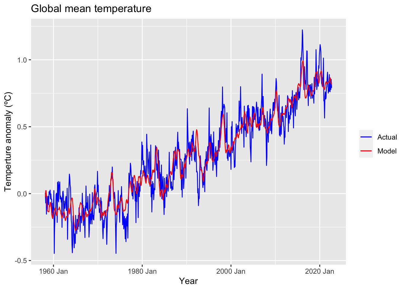
library(tidyverse)
library(fpp3)

# Load data and select data since 1970
HadCRUT <- read_csv("https://www.metoffice.gov.uk/hadobs/hadcrut5/data/current/analysis/diagnostics/HadCRUT.5.0.1.0.analysis.summary_series.global.monthly.csv")
HadCRUT <- HadCRUT %>%
        rename(time = "Time", Temperature = "Anomaly (deg C)") %>%
        select(time, Temperature)
HadCRUT$time <- as.Date(paste(HadCRUT$time, "-01", sep = ""))
HadCRUT <- HadCRUT %>%
        subset(time >= "1958-03-01")

co2 <- read_table("https://gml.noaa.gov/webdata/ccgg/trends/co2/co2_mm_mlo.txt",
                  col_names = FALSE, skip = 58)

co2 <- co2 %>%
        select(X1, X2, X4) %>%
        rename(Year = X1, 
               Month = X2, 
               CO2 = X4) %>%
        mutate(time = make_date(year = Year, 
                                month = Month, 
                                day = 1 )) %>%
        mutate(CO2_rf = 5.35*log(CO2/280)) %>%
        select(time, CO2_rf) %>%
        rename(CO2 = CO2_rf)



# Solar irradiance data

irradiance <- read_table("https://www2.mps.mpg.de/projects/sun-climate/data/SATIRE-T_SATIRE-S_TSI_1850_20220923.txt", 
                         col_names = FALSE, 
                         skip = 22) %>%
        rename(time = X1, 
               irradiance = X2) %>%
        select(time, irradiance) %>%
        mutate(daily = as.Date((time - 2396759), 
                               origin = as.Date("1850-01-01"))) %>%
        select(daily, irradiance) %>%
        mutate(time = floor_date(daily, "month")) %>%
        group_by(time) %>%
        summarize(irradiance = mean(irradiance, na.rm = TRUE)) %>%
        subset(time >= "1958-03-01") %>%
        rename(Solar =  irradiance)

# ENSO data

ENSO <- read_table("https://www.cpc.ncep.noaa.gov/data/indices/oni.ascii.txt")
ENSO$time <- seq.Date(from = as.Date("1950-01-01"), by = "month", length.out = nrow(ENSO))
ENSO <- subset(ENSO, time >= "1957-09-01") %>%
        rename(ENSO = ANOM) %>%
        select(time, ENSO)
ENSO$ENSO_lagged <- lag(ENSO$ENSO, 3)
ENSO <- ENSO %>%
        select(time, ENSO_lagged) %>%
        rename(ENSO = ENSO_lagged)

# Aerosols data

aerosols <- read_table("https://data.giss.nasa.gov/modelforce/strataer/tau.line_2012.12.txt",
                       skip = 3) %>%
        rename(time = "year/mon", Aerosols = global) %>%
        mutate_at(c("time", "Aerosols"), as.numeric) %>%
        select(time, Aerosols)

aerosols$time <- format(date_decimal(aerosols$time), "%Y-%m-01") %>%
        as.Date(aerosols$time, format = "%Y-%m-%d")
aerosols <- subset(aerosols, time >= "1955-10-01")

## Extrapolate out from 2012-09-01
length_out <- subset(ENSO, time >= "2012-10-01")
length_out <- length(length_out$time)

extrapolation <- data.frame(
        time = seq(from = as.Date("2012-10-01"), by = "1 month", length = length_out),
        Aerosols = "NaN"
)

aerosols <- rbind(aerosols, extrapolation)
aerosols$Aerosols <- as.numeric(aerosols$Aerosols)
aerosols <- imputeTS::na_interpolation(aerosols, option = "linear")
aerosols$Aerosols_lagged <- lag(aerosols$Aerosols, 18)
aerosols <- aerosols %>%
        select(time, Aerosols_lagged) %>%
        rename(Aerosols = Aerosols_lagged)
aerosols <- subset(aerosols, time >= "1958-03-01")

# Make data frame

df_list <- list(HadCRUT, co2, irradiance, ENSO, aerosols)
global_temp <- df_list %>%
        reduce(inner_join, by = "time") %>%
        mutate(date = decimal_date(time)) %>%
        mutate(time = yearmonth(time)) %>%
        as_tsibble(index = time)

# Create main model

fit_temp <- global_temp %>%
        model(TSLM(Temperature ~ CO2 + Solar + ENSO + Aerosols))

augment(fit_temp) %>%
        ggplot(aes(x = time)) +
        geom_line(aes(y = Temperature, colour = "Actual")) +
        geom_line(aes(y = .fitted, colour = "Model")) +
        labs(title = "Global mean temperature",
             x = "Year",
             y = "Temperture anomaly (ºC)") +
        scale_colour_manual(values = c(Actual = "blue",
                                       Model = "red")) +
        guides(colour = guide_legend(title = NULL))

Still a good match between actual and modelled temperature, with an adjusted R² of 0.8922. And no, there’s no reason for the switch from GISS. I merely wanted to try out a different temperature data set.

With that out of the way, the reason for this post is I decided to use this model to forecast near-term global temperature for the next five years. I also created a Shiny app where you can vary the forecast horizon from 1 to 10 years yourself. You can find it here. Enjoy.

In order to do this, I had to forecast the next five years of each independent variable, then run those forecasts through the model to predict mean global temperature. The forecast command runs each model 1,000 times, then gets the mean and 80% and 95% confidence intervals for each forecast. Here are the results for each predictive variable:

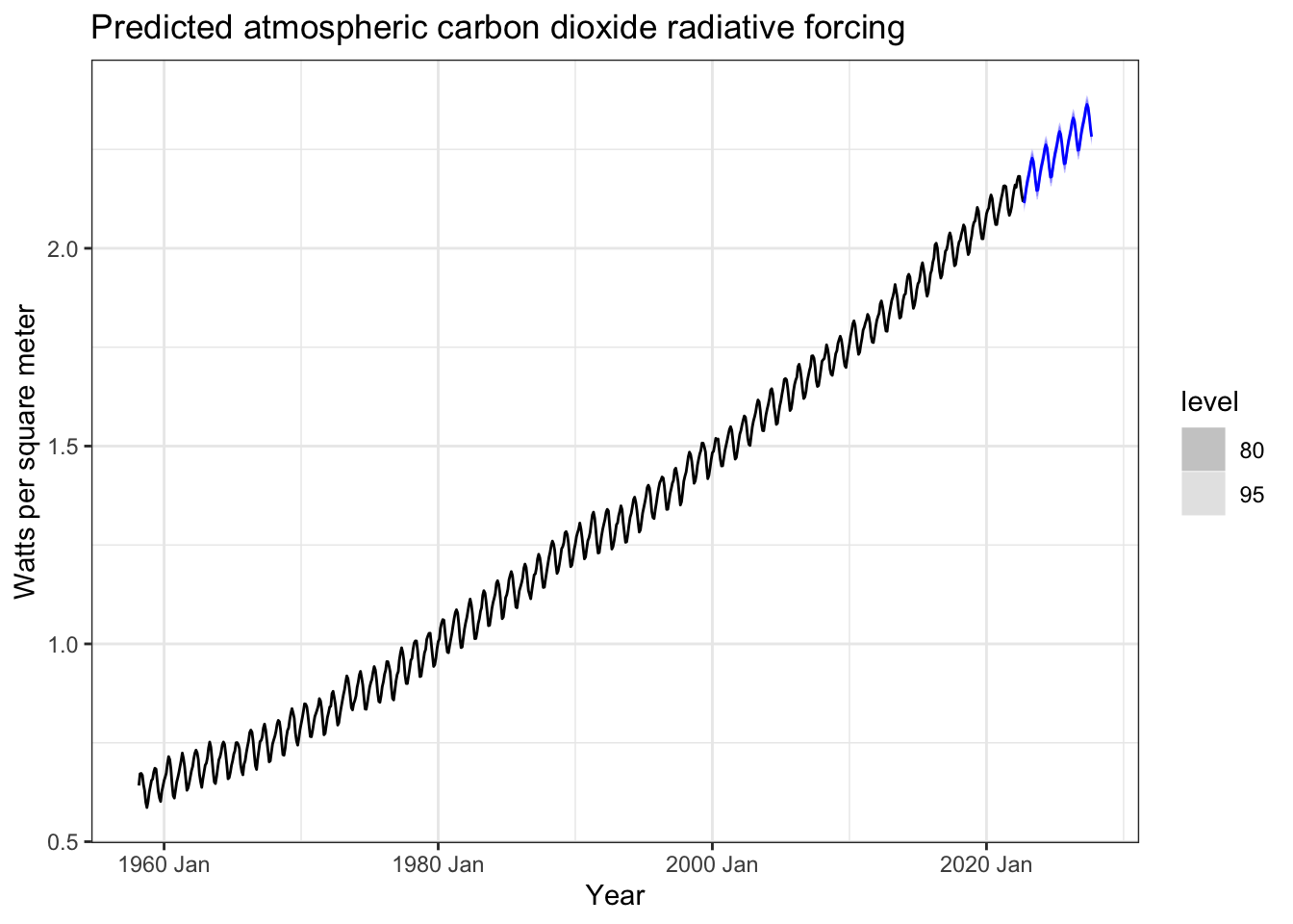
Carbon dioxide

In many ways, atmospheric CO2 is the easiest variable to forecast. Its trend is stable and the seasonal cycle has not changed over time. All I had to do was model a quadratic trend and add in the seasonal cycle.

Show the code

CO2_fit <- global_temp %>%
        model(TSLM(CO2 ~ trend() + I(trend()^2) + season()))

CO2_fc <- forecast(CO2_fit, h = 60)
pCO2 <- global_temp %>%
        autoplot(CO2) +
        autolayer(CO2_fc) +
        theme_bw() +
        labs(title = "Predicted atmospheric carbon dioxide radiative forcing",
             x = "Year",
             y = "Watts per square meter")
pCO2

As you can see, there is very little variation around the trend. You can barely see the confidence interval around the forecast line.

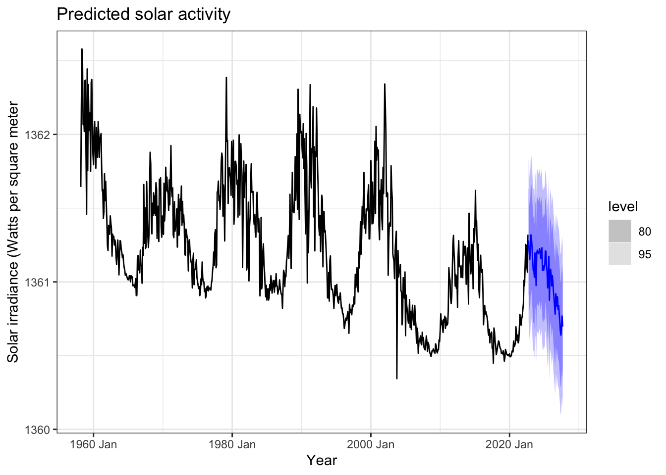
Solar irradiance

Again, this was an easy variable to model. There’s a trend, an annual cycle, and an 11-year cycle, which a Fourier model handled nicely.

Show the code

irradiance_fit <- global_temp %>%
        model(TSLM(Solar ~ trend() + 
                           season() + 
                           fourier(period = 132, K = 66)))

irradiance_fc <- forecast(irradiance_fit, h = 60)

pSolar <- global_temp %>%
        autoplot(Solar) +
        autolayer(irradiance_fc) +
        theme_bw() +
        labs(title = "Predicted solar activity",
             x = "Year",
             y = "Solar irradiance (Watts per square meter")
pSolar

There’s a bit less agreement between the forecasts but still a decent result.

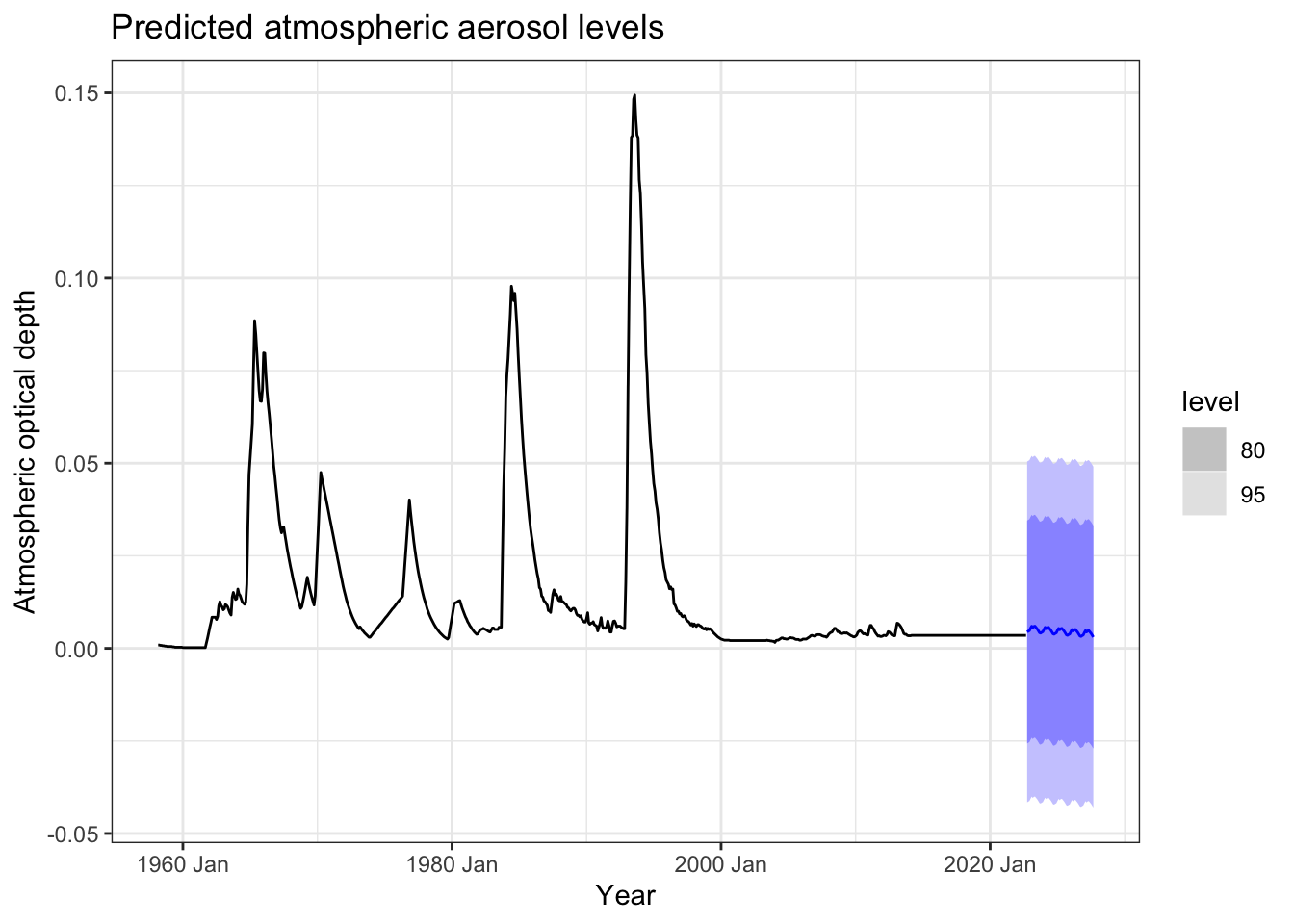
Aerosol optical depth

This is the one I’m least satisfied with, honestly. For one, the publicly available NASA data ends in 2012—I had to extrapolate from 2012 to include this in the model. If anyone has up-to-date AOD data, I’d love a link if you would send it to me. As it was, this was simple to model: trend plus seasonal cycle.

Show the code

aerosols_fit <- global_temp %>%
        model(TSLM(Aerosols ~ trend() + season()))


aerosols_fc <- forecast(aerosols_fit, h = 60)

pAerosols <- global_temp %>%
        autoplot(Aerosols) +
        autolayer(aerosols_fc) +
        theme_bw() +
        labs(title = "Predicted atmospheric aerosol levels",
             x = "Year",
             y = "Atmospheric optical depth")
pAerosols

El Niño/Southern Oscillation

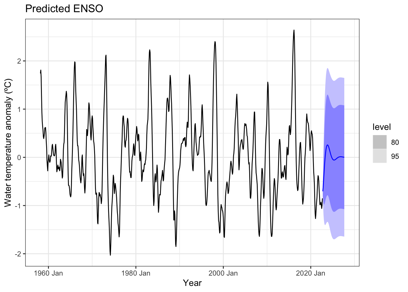
ENSO was the worst predictor to model. No trend to speak of (as expected with an oscillation) and seemingly random fluctuations from year to year with no clear seasonal or cyclical pattern. I finally went with a linear model with ARIMA errors, getting an linear trend with ARIMA(2, 0, 4) errors. I also tried a neural net model which showed similar results but needed way more computation time to get them. Either way, the prediction interval is wide enough to include everything from a major El Niño to a deep La Niña, highlighting the difficulty of modeling this phenomenon.

Show the code

ENSO_fit <- global_temp %>%
        model(ARIMA(ENSO ~ pdq(d = 0)))

ENSO_fc <- forecast(ENSO_fit, h = 60)
pENSO <- global_temp %>%
        autoplot(ENSO) +
        autolayer(ENSO_fc) +
        theme_bw() +
        labs(title = "Predicted ENSO",
             x = "Year",
             y = "Water temperature anomaly (ºC)")
pENSO

Predicted global mean temperature

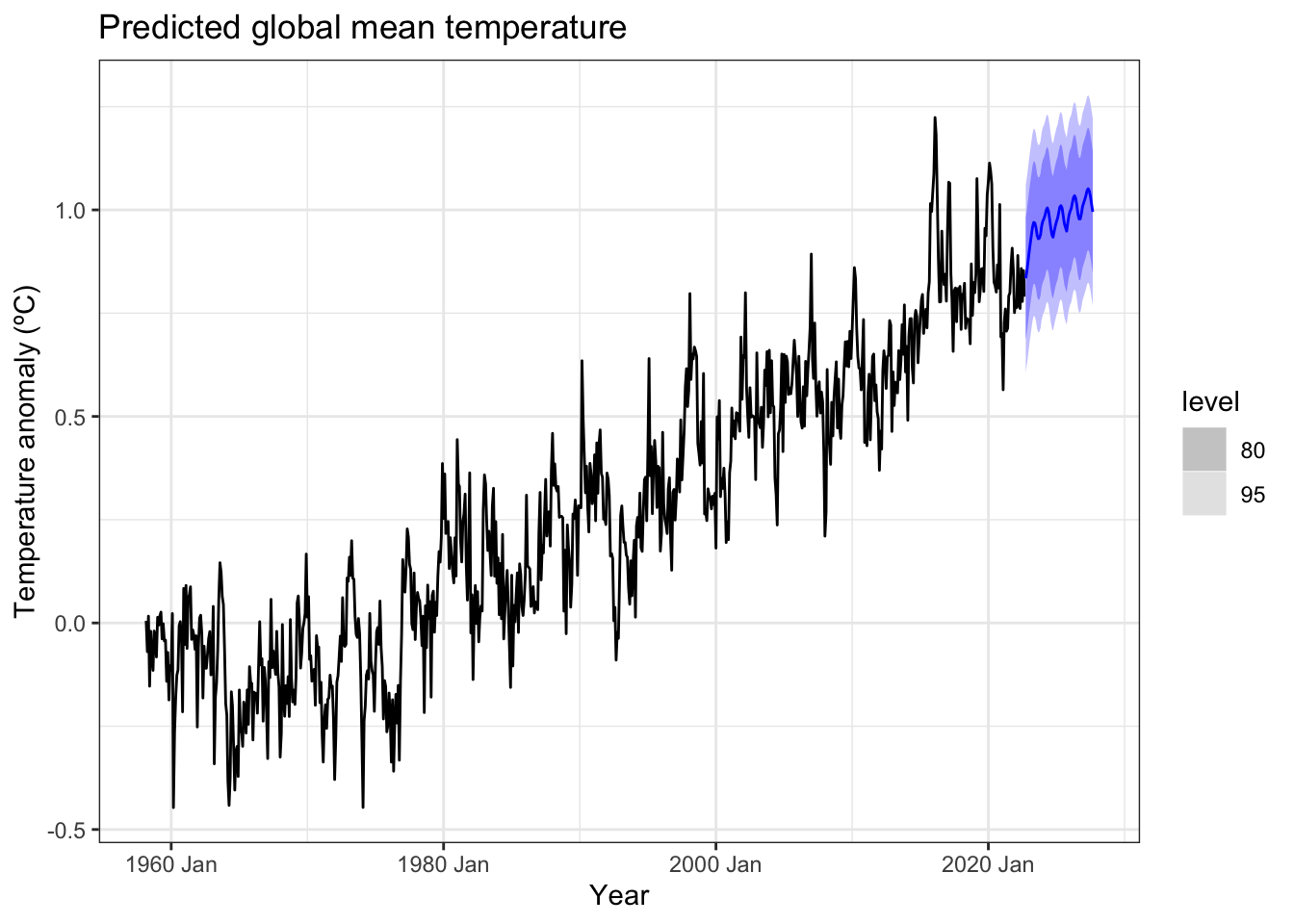
Finally, I brought the predicted mean values of all four variables into my main model to predict what global mean temperature may do in the near future.

Show the code

predictions_for_future <- scenarios(
                        CO2_fc <- forecast(CO2_fit, h = 60),
                        irradiance_fc <- forecast(irradiance_fit, h = 60),
                        aerosols_fc <- forecast(aerosols_fit, h = 60),
                        ENSO_fc <- forecast(ENSO_fit, h = 60),
                        Future = new_data(global_temp, 60) %>%
                                mutate(CO2 = CO2_fc$.mean,
                                       Solar = irradiance_fc$.mean,
                                       ENSO = ENSO_fc$.mean,
                                       Aerosols = aerosols_fc$.mean)
                )
                
# Forecast model for global temperatues
global_temp_forecast <- forecast(fit_temp,
                                 new_data = predictions_for_future$Future)
                
# Plot the forecast
p <- global_temp %>%
        autoplot(Temperature) +
        autolayer(global_temp_forecast) +
        theme_bw() +
        labs(title = "Predicted global mean temperature",
             x = "Year",
             y = "Temperature anomaly (ºC)")
p

As you can see, the model predicts continued warming, consistent with the linear trend since 1970. When that happens depends on the actual behavior of ENSO, which is capable of masking the overall trend over short time periods.

As I stated above, I created an app where you can play with the prediction horizon from 1 to 10 years and see how the predictions change depending on how far out you forecast. And if you want to see how the predictor variables interact in the main model, check out my previous post or just go to the Shiny app for that model as well.